PyCG 5: Inverse Kinematics

14 Aug 2019

Have you ever wondered how robotic arms control each of its segments so that its tip locates at an precise location? This is exactly one of the topics of inverse kinematics. Inverse kinematics is the mathematical process of recovering the movements of an object in the world from some other data, such as a film of those movements, or a film of the world as seen by a camera which is itself making those movements. In this case, the data we know is where the tip of the arm should be, and we would like to find out a way to position the arm segments correctly.

Forward kinematics

In order to solve this problem mathematically, we need a model for robotic arms. First, let’s consider a single arm segment. It is not hard to see that a single arm segment has two degrees of freedom, namely pitch and yaw (Euler angles). Denote the length, pitch and yaw of this arm segment by \(l_1\), \(p_1\) and \(y_1\), respectively. Assume its base is the origin, then its tip position is given by

\[\begin{equation*}\label{tip_one} \left\{ \begin{aligned} x_1 &= l_1 \cos(p_1)\cos(y_1)\\ y_1 &= l_1 \sin(p_1)\\ z_1 &= l_1 \cos(p_1)\sin(y_1) \end{aligned} \right. , \end{equation*}\]

which is fairly straightforward.

Now, what if there are two segments? One key observation is that now the second segment inherits some of the pitch and yaw values from the first segment, because even if the second segment stays fixed, if the first segment moves, the tip of the robotic arm will move as well. Thus, the actual pitch and yaw of the second segment is dependent on the first segment. Using similar notations, the tip position of the second segment relative to its base (i.e. the tip of the first segment) is given by

\[\begin{equation*}\label{tip_two} \left\{ \begin{aligned} x_2 &= l_2 \cos(p_1 + p_2)\cos(y_1 + y_2)\\ y_2 &= l_2 \sin(p_1 + p_2)\\ z_2 &= l_2 \cos(p_1 + p_2)\sin(y_1 + y_2) \end{aligned} \right. . \end{equation*}\]

To generalize this idea, assume that a robotic arm has \(n\) segments in total, where the \(i\)th segment has parameters \(l_i\), \(p_i\) and \(y_i\). If the first segment is based on the origin, the offsets of the \(i\)th segment with respect to the previous segment (denoted by \(\bm{o}_i\)) is given by

\[\begin{align*} \bm{o}_i = \begin{pmatrix} l_i\cos\left[ \sum_{t = 1}^{i} p_t \right]\cos\left[ \sum_{t = 1}^{i} y_t \right]\\ l_i\sin\left[ \sum_{t = 1}^{i} p_t \right]\\ l_i\cos\left[ \sum_{t = 1}^{i} p_t \right]\sin\left[ \sum_{t = 1}^{i} y_t \right] \end{pmatrix}, \end{align*}\]

and the end point of the entire system (denoted by \(\bm{e}\)) is given by

\[e = \sum_{i = 1}^{n} \bm{o}_i.\]

Analyzing the inverse problem

It is very difficult to solve this problem in closed form because for \(n\) arm segments, there are \(2n\) parameters, but the only information we know is merely three digits (the tip position in 3D space). Therefore, the only solution left seems to be an iterative approximation. However, since robotic arms in real life tend to move smoothly between two locations, an iterative solution will be desirable because it will have smooth transitions between two states as well.

If we concatenate all parameters in this model into one long vector \(\bm{u}\), where

\[\begin{align*} \bm{u} &= \left( p_1, p_2, \ldots, p_n, y_1, y_2, \ldots, y_n \right)^T\\ &= \left( u_1, u_2, \ldots, u_n, u_{n+1}, u_{n+2}, \ldots, u_{2n} \right)^T, \end{align*}\]

then we can conveniently say

\[\bm{e} = f(\bm{u}).\]

The Jacobian matrix \(\bm{J}_f(\bm{u})\) provides the best linear approximation of \(f\) near the point \(\bm{u}\). The matrix itself is given by

\[\bm{J}_f(\bm{u}) = \begin{bmatrix} \frac{\partial f_x}{\partial{u_1}} & \frac{\partial f_x}{\partial{u_2}} & \cdots & \frac{\partial f_x}{\partial{u_{2n}}}\\ \frac{\partial f_y}{\partial{u_1}} & \frac{\partial f_y}{\partial{u_2}} & \cdots & \frac{\partial f_y}{\partial{u_{2n}}}\\ \frac{\partial f_z}{\partial{u_1}} & \frac{\partial f_z}{\partial{u_2}} & \cdots & \frac{\partial f_z}{\partial{u_{2n}}} \end{bmatrix},\]

and the linear approximation around \(\bm{u}\) writes

\[f(\bm{u} +\bm{\Delta}) \approx f(\bm{u}) + \bm{J}_f(\bm{u}) \bm{\Delta}.\]

When we begin solving the inverse kinematics problem, the robotic arm must have some initial \(\bm{u}\). In order to move its tip towards another location, we cut the desired path into many smaller paths and make use of this linear approximation for each of those short paths. That is, we know what \(f(\bm{u} +\bm{\Delta})\), \(f(\bm{u})\), and \(\bm{J}_f(\bm{u})\) are, and we would like to solve for \(\bm{\Delta}\). We can write

\[\bm{J}_f(\bm{u})\bm{\Delta} = f(\bm{u} +\bm{\Delta}) - f(\bm{u}),\]

but we cannot solve this equation in closed form because \(\bm{J}_f(\bm{u})\) is not a square matrix. We can only get an approximation by using linear least square methods, which minimizes \(\lVert \bm{J}_f(\bm{u})\bm{\Delta} - \left[ f(\bm{u} +\bm{\Delta}) - f(\bm{u}) \right] \rVert\) for \(\bm{\Delta}\). The least square solution of \(\bm{\Delta}\) can be computed using Moore–Penrose inverse (also possible to use QR decomposition). Then we can update the new parameters with \(\bm{u} + \bm{\Delta}\).

Demo

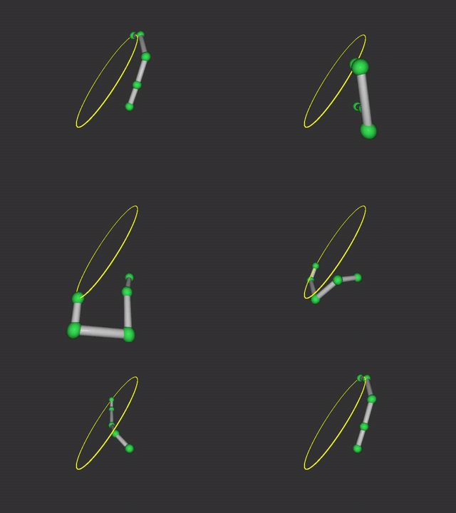
After deriving the numerical solution to this problem, it is trivial to write a OpenGL demo for it. Here is a little hint for creating a smooth and accurate animation. The iterative step size is set to be uniform at first, but because sometimes the step size maybe too big to have a good linear approximation, we need to shrink the step size until we can have an ideal solution. As a result, the final sequence of parameters we get may not have a uniform spacing. In order to generate smooth animations with uniform spacing, I applied linear interpolation across the parameter sequence.

The source code of the demo is on GitHub.

Basic usages:

• Use mouse and “wasd” to look/walk around
• Press Esc to exit
• Press “p” to take screenshots

Futher reading

• Mathematics for Inverse Kinematics
• Buss, Samuel R. “Introduction to inverse kinematics with jacobian transpose, pseudoinverse and damped least squares methods.” IEEE Journal of Robotics and Automation 17.1-19 (2004): 16.